This blog post gives a summary of the article Making Deep Q-learning Approaches Robust to Time Discretization.
A bit of motivation
Have you ever tried training a Deep Deterministic Policy Gradient [3] agent on the OpenAI gym Bipedal Walker [2] environment? With very little hyperparameterisation, you can get it to kind of work, and you would probably obtain something of the sort:
Now, have you ever tried to do it with a framerate of 1000 FPS instead of the usual 50 FPS? Kind of crazy, but things should only be easier. We are just providing our agent with a much smaller reaction time, and this should only improve its performance. If you were able to react 20 times faster than you normally would, you would expect to become much better at everything you do, not much worse.
Strange, the agent is not learning anything anymore… And if you perform the same experiment on different environments, you will get the same kind of results. There seems to be something wrong with Q-learning when the framerate time becomes arbitrarily high.
This is not at all the behavior we expect for a reinforcement learning algorithm. Imagine starting to play to a new video game. Your learning behavior would be exactly the same if the game render 50 frame per second or 500 frame per second. This is because the underlying learning process is independant of the time discretization. We expect the same thing from a RL method!
Is that a real problem in practice? One could argue that most of the time, we are only using a single time discretization. That’s true. But it suggests that you will always have to tune every hyperparameter on a new problem in order to adapt them to the time discretization. The algorithms will be extremely sensitive to hyperparameter choice, and it will take more time to make an algorithm work in practice on a new problem. On the contrary, if the learning algorithm is time-discretization invariant, this means there is one less thing to adapt. Thus, it should be easier to find reasonnable hyperparameter, and the method should be more stable and robust.
Outline
Before going into details, here is a very short summary of our work:
We study the influence of time discretisation on Q-learning and DDPG: We show that in order to obtain a well-behavied algorithm, we should change three aspects of the method:
- The architecture of the network approximating the Q-function must be adapted to the time discretization, such that its outputs are of the proper order of magnitude.
- The exploration strategy must depend on the time discretization and be time coherent.
- The learning rates must be adapted to the time discretization.
With these three ingredients, the algorithm converge when the time discretization goes to 0 to a well defined “continuous algorithm”. This is a necessary step towards invariance to time discretization.
A crash course on approximate Q-learning
Click if you are not familiar with Q-learning
In the following section, some elementary notions of reinforcement learning are given, as well as a reminder on *Q-learning*. If you are already familiar with the domain, you may want to directly skip to the next section. ## Markov Decision Process We are going to work in the context of *Markov Decision Processes*. In this context, the observations received by the agent form a complete description of the state of the environment. To make things formal, a *Markov Decision Process* $\mathcal{M}$ is defined as a quadruplet $(\mathcal{S}, \mathcal{A}, \mathcal{P}, \mathcal{R})$, where - $\mathcal{S}$ is the state space, or observation space of the environment - $\mathcal{A}$ is the action space of the agent - $\mathcal{P}$ is the transition kernel of the environment. $P(s'|s, a)$ represents the probability for the agent of landing in state $s'$ after executing action $a$ in state $s$. - $\mathcal{R}$ is the reward function. $R(s, a)$ represents the reward obtained by the agent when executing action $a$ in state $s$. To make things slightly simpler, we assume that the reward is deterministic. The agent interacts with the environment through a (potentially stochastic policy $\pi$, where $\pi(a|s)$ represents the probability for the agent of executing action $a$ in state $s$. ## Policy and Value function The goal of the agent is to find a policy $\pi$ that maximizes the expected sum of weighted rewards across all subsequent timesteps. Formally, let's define the value function as $$ V^\pi(s) = \mathbb{E}_{(sa)_t \sim \pi} \left[\sum\limits_{t=0}^{+\infty}\gamma^t R(s_t, a_t)\mid s_0=s \right] $$ where the expectation is over trajectories sampled by using policy $\pi$ to interact with the environment. The goal of the agent is to find a policy $\pi^\*$ such that for all policies $\pi$, for all state $s$, $V^{\pi^*}(s) \geq V^\pi(s)$. ## Discount factor and time horizon You may notice that a *discount factor* $\gamma$ was introduced in the definition of $V^\pi$. Besides providing existence of the value function, this parameter can be interpreted as a preference for the present of the agent. Informally, $\gamma$ introduces a notion of temporal horizon, $T = \frac{1}{1 - \gamma}$, and the agent roughly optimizes the sum of rewards up to a temporal horizon of order $T$. Having a $\gamma$ of $.9$ thus roughly means looking about $10$ environment steps into the future. ## Q-learning: Learning the optimal state-action value function $Q^\*$ *Q-learning* is a way of computing an approximation of this optimal policy. To explain how it works, we first need to introduce the notion of *state-action value function* \begin{equation} Q^\pi(s, a) = \mathbb{E}\_{(sa)\_t \sim \pi} \left[\sum\limits\_{t=0}^{+\infty}\gamma^t R(s\_t, a\_t)\mid s\_0=s, a\_0=a \right]. \end{equation} If one succeeds in computing the *optimal state-action value function* $Q^\* = Q^{\pi^*}$, one can directly obtain a deterministic optimal policy as \begin{equation} \pi(a | s) = \delta\_{\text{argmax}\_a Q^\*(s, a)}. \end{equation} The optimal state-action value function verifies the *optimal Bellman equation* \begin{equation} Q^\*(s, a) = R(s, a) + \gamma \mathbb{E}\_{s' \sim P(.|s, a)} \left[\max\limits\_{a'} Q^*(s', a')\right]. \end{equation} When both the state and action spaces are discrete, this equation gives us an intuitive way of iteratively building new estimations of $Q^*$, starting from an original guess $Q^0$, and from a sequence of observations and actions $(sa)_t$, obtained using an exploration policy $\pi^\text{explo}$: 1. Sample the next transition from the sequence $(s_t, a_t, s_{t+1})$. 2. Compute a new estimate of the state action value function at $(s_t, a_t)$ by using the left-hand side of the optimal Bellman equation \begin{equation} \tilde{Q}^{t+1}(s_t, a_t) = R(s_t, a_t) + \gamma \max_{a'} Q(s', a') \end{equation} 3. Update the estimate $Q^t$ at point $(s_t, a_t)$ by using a weighted average of the old and new estimate of $Q$ \begin{equation} Q^{t+1}(s_{t+1}, a_{t+1}) = (1 - \alpha_{t+1}) Q^t(s_{t+1}, a_{t+1}) + \alpha_{t+1} \tilde{Q}^{t+1}(s_t, a_t). \end{equation} 4. Update $t$ to $t+1$ and go to 1. Under suitable conditions on the $\alpha$'s, this procedure can be shown to converge to the true optimal state-value function. This is *tabular Q-learning*! ## Deep-Q-learning: Approximating $Q^\*$ via gradient descent When facing continuous state space, we would like to approximate $Q^\*$ using a parametric function approximator $Q_\theta$. To this end, we can modify the previous learning procedure by replacing $3$ by - Update the estimate $Q_{\theta_t}$ by performing one gradient step to minimize the quadratic error between the current estimate and the new estimate, considering the new estimate as independent of $\theta$ \begin{equation} \theta\_{t+1} = \theta\_t - \alpha\_t (Q\_{\theta\_t}(s\_t, a\_t) - \tilde{Q}\_{\theta\_t}(s\_t, a\_t)) \partial\_\theta Q\_{\theta\_t}(s\_t, a\_t). \end{equation} Unfortunately this algorithm is no longer guaranteed to converge. Still, it performs relatively well in practice, provided you use a couple of tricks to make it scale (see e.g. [4, 5]). In sum, as a reinforcement learning algorithm, Q-learning displays three key properties: 1. It is *temporal difference based*. More precisely it revolves around the use of the *optimal Bellman Equation*. 2. It is *model free*. It does not need to know, or to model the dynamic of the environment to learn. 3. It is *off-policy*, i.e. it learns a different policy than the one it actually uses to produce its training trajectories.What is continuous time Reinforcement Learning, and why does it matters
Click if you want to know more about continuous-time reinforcement learning.
To study the behavior of Q-learning when the framerate goes to $+\infty$, or equivalently the discretization timestep goes to $0$, we must first define a notion of discretized MDPs. To that end, we will introduce a restricted class of *continuous* environments, that will yield a familly of discretized environments, one for each discretization timestep. ## Continuous environments and discretized MDPs The continuous environments we define are quadruplets $(\mathcal{S}, \mathcal{A}, F, R)$ where - $\mathcal{S}$ is a *continuous* state space. - $\mathcal{A}$ is an action space. - $F$ a dynamic transition function, such that state action trajectories verify the ordinary differential equation \begin{equation} ds\_t/dt = F(s\_t, a\_t). \end{equation} - A *reward density* which associates a density of reward to each state action pair. This environment is not an actual MDP, since it does not provide a well defined transition kernel. From this definition, for any $\deltat > 0$, we can define an associated *discretized MDP* $\mathcal{M}\_{\deltat} = (\mathcal{S}\_{\deltat}, \mathcal{A}\_{\deltat}, P\_{\deltat}, R\_{\deltat})$ where - $\mathcal{S}\_{\deltat} = \mathcal{S}$ - $\mathcal{A}\_{\deltat} = \mathcal{A}$ - $P\_{\deltat}(s' \mid s, a) = \delta\_{s + F(s, a) \deltat}(s')$ - $R\_{\delta_t}(s, a) = R(s, a) \deltat$ (we will come back to that definition below). To avoid having to deal with the burden of defining stochastic policies in continuous time, we restrict ourselves to deterministic exploitation policies, i.e. policies of the form $\pi(a\mid s) = \delta_{\tilde{\pi}(s)}$ where $\tilde{\pi}$ is a function of states. Our aim is then to analyse the behavior of Q-learning when $\deltat$ becomes small. ## Physical time/Number of steps In a standard reinforcement learning setup, you have an intrinsic notion of time ellapsed which is the number of steps during which the agent interacted with the environment. In a discretized environment, there is a competing notion of time, which is the actual amount of time the agent spent interacting with the environment. Ideally, we would like our algorithms to scale in term of *physical time*. This means that, for any $\deltat$, we would like our agent to have learnt approximately the same thing, after the same amount of physical time spent in the environment. This property can only hold in term of physical time: after interacting for the same amount of steps with two different discretization of the same environment, the diversity of trajectories encountered by the two agents are going to be radically different, and we thus cannot expect to obtain the same perfomance. The two notions of time described are related through \begin{equation} \text{physical time} = \text{number of steps} \times \deltat. \end{equation} ## Value function, discount factor and time horizon in continuous time For each of our discretized MDPs, we need to define a specific discount factor $\gamma\_{\deltat}$. Indeed, if we keep the discount factor constant across time discretizations, our agent is going to become increasingly shortsighted. This is easily seen if you look at the time horizon in physical time. The time horizon in physical time is $\frac{\deltat}{1 - \gamma\_{\deltat}}$. If $\gamma\_{\deltat}$ is independent of $\deltat$, as $\deltat$ goes to zero, the time horizon goes to $0$, and the agent only optimizes its current reward. To properly define $\gamma$, let's look at the standard definition of the value function in continuous settings: \begin{equation} V^\pi(s) = \mathbb{E}\_{(sa)\_t \sim \pi}\left[\int\_0^{+\infty} \gamma^t R(s\_t, a\_t) dt \mid s_0 = s\right]. \end{equation} For a given $\deltat$, one can discretize this equation and obtain \begin{equation} V^\pi_{\deltat}(s) = \mathbb{E}\_{(sa)\_t \sim \pi}\left[\sum\limits\_{k = 0}^{+\infty} (\gamma^{\deltat})^k R(s\_{k \deltat}, a\_{k \deltat})\deltat \mid s_0 = s\right]\approx V^\pi(s). \end{equation} This directly suggests setting $\gamma\_{\deltat} = \gamma^{\deltat}$, and explains the scaling of rewards in the discretized MDP. With this definition of $\gamma\_{\deltat}$, one can compute the corresponding physical time horizon for each $\deltat$ \begin{equation} T_{\deltat} = \frac{\deltat}{1 - \gamma^{\deltat}} = - \frac{1}{\log \gamma} + O(\deltat) \end{equation} thus yielding a non trivial time horizon as $\deltat$ goes to $0$, and physical time horizon close to this this value in near continuous environments.What’s wrong with near continuous Q-learning?
We are now ready to study what is going wrong with near continuous time Q-learning.
There is no continuous time Q-function
One of the two major issues with Q-learning in near continuous time is that, as $\deltat$ goes to $0$, the state action value function depends less and less on its action component, which is the component that makes one able to rank actions, and thus improve the policy. Intuitively, as $\deltat$ goes to $0$, the effect of doing action $a$ instead of action $a’$ for a duration $\delta t$, then following a fixed policy has a negligible effect on the overall state trajectory, and consequently on the expected return, thus making $Q^\pi_{\deltat}(s, a)$ very close to $Q^\pi_{\deltat}(s, a’)$. Besides, the smaller the $\deltat$, the smaller the effect.
Formally, writting $Q^\pi_{\deltat}$ as \begin{equation} Q^\pi_{\deltat}(s_t, a_t) = R(s_t, a_t) \deltat + \gamma^{\deltat} V^\pi_{\deltat}(s_{t + \deltat}) \end{equation} and performing a first order Taylor expansion yields \begin{align} Q^\pi_{\deltat}(s_t, a_t) = V^\pi_{\deltat}(s_t) + \deltat \left(R(s_t, a_t) + \log(\gamma) V^\pi_{\deltat}(s_t) + \partial_s V^\pi_{\deltat}(s_t) F(s_t, a_t)\right) + o(\deltat) = V^\pi_{\deltat}(s_t) + O(\deltat) \end{align} and as $\deltat$ goes to $0$, $Q^\pi_{\deltat}$ collapses to $V^\pi_{\deltat}$, thus becoming independent of actions. When $\deltat$ is close to $0$, the effect of actions on $Q^\pi_{\deltat}$ is expected to be about $\deltat$ times smaller than the effect of states. When learning $Q$ for small $\deltat$, it is likely that capturing the state dependency will be easy, but capturing the comparatively very small action dependency, which is the interesting component, will be hard.
To illustrate this effect we display the evolution of the relative size of $Q - V$ and $V$ on the pendulum environment, while learning using DQN [5]. On this simple environment, DQN is still able to learn, even with a relatively small $\deltat$, but the order of magnitude of the action dependency of $Q$ varies considerably during training.
Exploration and time discretization
The second failing component of many Q-learning based approaches is the exploration mechanism. In discrete action setups, the most common exploration scheme used is $\varepsilon$-greedy exploration, which consists in selecting the maximizer of the current estimate of $Q$ with probability $1 - \varepsilon$, and of picking an action at random with probability $\varepsilon$. The problem is that, as $\deltat$ goes to $0$, $\varepsilon$ -greedy exploration explores less and less, and in the limit of infinitesimal $\deltat$, does not explore at all.
To get a grasp of why this happens, let’s look at a very simple example. Take a continuous environments of the form \begin{equation} ds_t / dt = a_t \end{equation} with $a_t \in \{-1, 1\}$. If we apply the most exploratory form of $\varepsilon$-greedy exploration, with $\varepsilon=1$ to discretized versions of this environment, we obtain the following approximative expression for the value of the state at any instant $t$ \begin{equation} s_t = s_0 + \sum\limits_{k=0}^{\frac{t}{\deltat}} a_k \deltat \end{equation} with the $a_k$’s being independent uniform random variables. Now, applying the central limit theorem, one obtains the following approximation \begin{equation} s_t = s_0 + \mathcal{N}\left(0, t \deltat\right). \end{equation} As $\deltat$ goes to $0$, the variance of the right-hand-side normal variable goes to $0$, and consequently, $s_t$ goes to $s_0$.
This is quite visible experimentally. For instance, let’s have a look at the pendulum environment. If we use $\varepsilon$-greedy exploration, with $\varepsilon = 1$ with $\deltat = 0.05$, we obtain the following behaviour
Now, if we use the exact same policy with $\deltat = 0.0001$, the exploration behaviour is tenuous
Can we fix it?
Click if you want to know how to fix it!
We would now want to build a version of Q-learning that provides better invariance guarantees than standard approaches, and notably to work with small and very small $\deltat$'s. ## Methodology A necessary property for an algorithm to provide invariance, or quasi invariance to changes in $\deltat$, is that there should exist a limit algorithm, that makes sense in continuous time, when dealing with a continuous environment. This means that all the quantities that we use should admit continuous time limits, that still bear the same information as their discrete counterpart. Our methodology is thus to define: - A quantity to learn, that would replace the usual state-action value function, but would admit a continuous time limit that still contains information on the ranking of actions. - A way to learn this quantity, which provides meaningful parameter trajectories, i.e. learning trajectories that do not diverge instantaneously, and move away from their initialization, as $\deltat$ goes to $0$. - An exploration method that do explore in continuous time, and whose exploration should be nearly $\deltat$ invariant. ## What to learn? As mentionned previously, the continuous time limit of the state-action value function does not bear the information about the ranking of actions we are interested in. The part of the Q-function that we are interested in is the $O(\deltat)$ part of $Q$ that makes it differ from the V-function. We can directly try to learn this quantity, that we call the normalized advantage function \begin{equation} A^\pi\_{\deltat}(s, a) = \frac{Q^\pi\_{\deltat}(s, a) - V^\pi\_{\deltat}(s)}{\deltat}. \end{equation} The normalized advantage function admits a continuous time limit \begin{equation} A^\pi(s, a) = R(s, a) + \log(\gamma) V^\pi(s) + \partial\_s V^\pi(s) F(s, a) \end{equation} which contains the necessary information to perform policy improvement, namely, if there exists a pair $(s\_0, a\_0)$ such that $A^\pi(s\_0, a\_0) > 0$, then the policy $\pi'$ which only differs from $\pi$ by selecting $a\_0$ in state $s\_0$ is better than $\pi$. ## How to learn it? Now that we know what quantity we want to learn, we are only left with the burden of finding a way to learn it. Fortunately, from the usual Bellman equation on the state-action value function, equations on the normalized advantage function and the value function can be derived: \begin{equation} A^\pi\_{\deltat}(s\_t, a\_t) = R(s\_t, a\_t) + \frac{\gamma^{\deltat} V^\pi\_{\deltat}(s_{t + \deltat}) - V^\pi\_{\deltat}(s\_t)}{\deltat} \end{equation} \begin{equation} A^\pi\_{\deltat}(s, \pi(s)) = 0. \end{equation} Corresponding optimal equations can easily be derived. When trying to learn $A^\pi\_{\deltat}$ and $V^\pi\_{\deltat}$, from parametric function $A\_\theta$ and $V\_\phi$, we can directly verify the second equation by using a neural network to represent a function $\bar{A}\_\theta$, then computing $A\_\theta(s, a) = \bar{A}\_\theta(s, a) - \bar{A}\_\theta(s, \pi(s))$. For the second equation, assuming an exploratory trajectory $\tau=(sa)\_t$, we can use TD-like updates, to get the following parameter equations, for learning rates $\alpha\_V \deltat^\beta$ and $\alpha\_A \deltat^\beta$ \begin{equation} \delta A(s\_t, a\_t) \leftarrow A\_{\theta}(s\_t, a\_t) - \left(R(s\_t, a\_t) + \frac{\gamma^{\deltat} V_\phi(s_{t + \deltat}) - V\_\phi(s\_t)}{\deltat}\right) \end{equation} \begin{equation} \theta \leftarrow \theta - \alpha\_A \deltat^\beta \delta A(s\_t, a\_t) \partial\_\theta A\_\theta(s\_t, a\_t) \end{equation} \begin{equation} \phi \leftarrow \phi - \alpha\_V \deltat^\beta \delta A(s\_t, a\_t) \partial\_\theta V\_\theta(s\_t). \end{equation} The final step is to properly set our learning rates, such that the parameter updates behave nicely in near continuous time. The only way to obtain proper trajectories is to set $\beta = 1$. More precisely: - If $\beta = 1$, parameter trajectories converge to continuous trajectories that satisfy a non trivial ordinary differential equation. - If $\beta > 1$, parameter trajectories remain closer and closer to their initialization as $\deltat$ goes to $0$. - If $\beta < 1$, parameter trajectories can diverge in infinitesimal time, as $\deltat$ goes to $0$. Given proper exploration trajectories, we now have an algorithm that is able to learn a quantity that contains some information about the ranking of actions, even in continuous time. ## How to explore? What we want is an exploration strategy that, contrary to $\varepsilon$-greedy, do explore, even when $\deltat$ goes to $0$. The key here is to define a temporally coherent exploration process: if a possibility is explored at time $t$, we should consider keeping exploring it at time $t+\deltat$. Fortunately, for continuous action spaces, such an exploration process already exists [3], and simply consists in adding the discretization of a continuous stochastic process to action. The chosen continuous process is an *Ornstein Uhlenbeck* process, defined by the stochastic differential equation \begin{equation} dX_t = - \theta X_t + \sigma dB_t \end{equation} where $B_t$ is a standard brownian motion. You can think of this process as the limiting process of \begin{equation} X_{t + \deltat} = (1 - \theta \deltat) X_t + \sigma \sqrt{\deltat}\mathcal{N}(0, I). \end{equation} Intuitively, $\theta$ is a recall parameter, it brings the process back to the origin when $X$ gets far, while $\sigma$ is a noise amplitude parameter. To have an idea of what difference this makes in term of temporal coherence, let us visualize examples of $2$-d processes, where one is an OU process, while the other is obtained by generating independent gaussian noises at each timestep. *Independent gaussian noise:*  *Ornstein Uhlenbeck noise:* Results
With all the above remarks in hand, we can devise an algorithm, which we will refer to as Deep Advantage Updating (DAU), due to its resemblance to Advantage Updating [1], that should be more resilient to changes in framerate than standard algorithms. We are left to test this statement experimentally.
As a first qualitative validation, we test the resilience of both DDPG and DAU to changes in framerate on the simple pendulum environment from OpenAI gym.
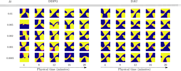
To that end, we display the policy in phase space learnt after fixed physical times, for different values of $\deltat$.
We also test quantitatively the resilience wrt to $\deltat$ on a variety of environments:
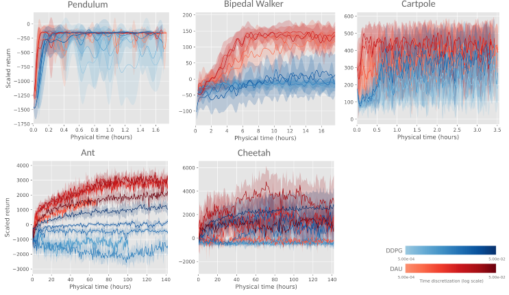
Overall, DAU is substantially more resilient to changes in $\deltat$ than DDPG. On many environments, it already outperforms DDPG for the standard $\deltat$, as the standard framerate is already quite high (typically $20$ or $50$ FPS).
Finally, coming back to our motivating example, what happens when training using DAU on the Bipedal walker environment, with different framerates. With the usual framerate, DAU behaves approximately the same as DDPG:
Now, with a framerate $20$ times larger:
DAU succeeds in learning a decent behavior, even with a vastly larger framerate !
As an important aside, do note that you can only hope to achieve invariance in term of physical time, not number of steps. This means that when you are training with a $\deltat$ $10$ times smaller than the standard $\deltat$, you must train for $10$ times the usual training time if you hope to obtain the same results. This makes results for very low $\deltat$’s costly to obtain.
References
- [1] BAIRD III, Leemon C. Advantage updating. WRIGHT LAB WRIGHT-PATTERSON AFB OH, 1993.
- [2] Brockman, G., Cheung, V., Pettersson, L., Schneider, J., Schulman, J., Tang, J., & Zaremba, W. (2016). Openai gym. arXiv preprint arXiv:1606.01540.
- [3] Lillicrap, T. P., Hunt, J. J., Pritzel, A., Heess, N., Erez, T., Tassa, Y., … & Wierstra, D. (2015). Continuous control with deep reinforcement learning. arXiv preprint arXiv:1509.02971.
- [4] Tesauro, G. (1995). Temporal difference learning and TD-Gammon. Communications of the ACM, 38(3), 58-68.
- [5] Mnih, V., Kavukcuoglu, K., Silver, D., Rusu, A. A., Veness, J., Bellemare, M. G., … & Petersen, S. (2015). Human-level control through deep reinforcement learning. Nature, 518(7540), 529.